16 Recurrent Neural Networks
Recurrent neural networks are models that capture the dynamics of sequences via recurrent connections, which can be thought of as cycles in the network of nodes.
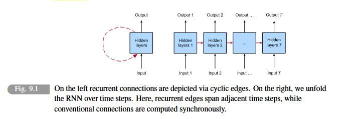
Recurrent neural networks are unrolled across time steps with the same underlying parameters applied at each step. While the standard connections are applied synchronously to propagate each layer’s activations to the subsequent layer at the same time step, the recurrent connections are dynamic, passing information across adjacent time steps.
RNNs can be thought of as a feedforward network where each layer’s parameters are shared across time steps.
Inputs consist of an ordered list of feature vectors x_1, \ldots, x_r where each feature vector x_t is indexed by a time step t. We assume that entire sequences are sampled independently, but we cannot assume anymore that the data arriving at each time step are independent of each other. Furthermore, we sometimes wish to predict a fixed target y while having as input a sequence, sometimes we wish to predict a sequence of targets (y_1, \ldots, y_r) given a fixed input. Other times, our goal is to predict sequentially structured targets based on sequentially structured inputs. Such sequence-to-sequence tasks take two forms:
- aligned: where the input at each time step aligns with a corresponding target (e.g. part of speech tagging)
- unaligned: where input and target do not necessarily exhibit a step-for-step correspondence (e.g. machine translation)
16.1 Sequence models
We wish to estimate the joint probability of an entire sequence. These functions are called sequence models. We will use as examples words, as the field of sequence modeling has been driven so much by natural language processing.
We can reduce language modeling to autoregressive prediction y decomposing the joint density of a sequence p(x_1, \ldots, x_r) into the product of conditional densities in a left-to-right fashion by applying the chain rule of probability P(x_1, ..., x_r) = P(x_1) \prod_{t = 2}^T P(x_t | x_{t-1}, ... ,x_1) The autoregressive model will output a full probability distribution over the vocabulary of words.
16.1.1 Markov models
Whenever we can throw away the history beyond the previous t steps without any loss in predictive power, we say that the sequence satisfies a Markov condition: the future is conditionally independent of the past, given the recent history. We talk about k^{th}-order Markov models, with t = k. The factorization becomes a product of probabilities of each word given the previous word: P(x_1, ..., x_r) = P(x_1) \prod_{t = 2}^T P(x_t | x_{t - 1}) With discrete data (like words), P(x_t | x_{t-1}) simply counts the number of times that each word has occurred in each context. The k we define will condition how much we want to approximate the sequence model:
- If we consider only the previous word, we are making a unigram model
- If we consider only the two previous words, we are making a bigram model
- and so on (n-gram models)
16.1.2 Evaluation of a language model
We might measure the quality by computing the likelihood of the sequence, but this is a number that is hard to understand, and we cannot compare sequences with different lengths, as shorter sequences are more frequent than longer ones. Instead, we use information theory concepts: a better language model should allow us to spend fewer bits in compressing a sequence. So we can measure the performance by the cross-entropy loss averaged over all the n tokens of a sequence \dfrac{1}{n} \sum_{ t = 1}^n - \log P (x_t | x_{t - 1}, \dots, x_1) Usually, we use the perplexity measure, that is, the exponential of the cross-entropy loss previously described. \text{Perplexity} = \exp \left( \dfrac{1}{n} \sum_{ t = 1}^n - \log P (x_t | x_{t - 1}, \dots, x_1) \right)
- In the best case scenario, the model always predicts the probability of the target token as 1. In this situation, the perplexity is 1
- In the worst case scenario, the model always predicts the probability of the target token as 0. In this situation, the perplexity is positive infinity.
16.2 Recurrent Neural Networks
The problem with Markov Models is that increasing the order k would also increase exponentially the number of model parameters, as we need to store |\mathcal{V}|^n numbers for a vocabulary set \mathcal{V}. Hence, rather than modeling P(x_t | x_{t-1}, \ldots, x_{t-n+1}) it is preferable to use a latent variable model, introducing an hidden state: P(x_t | x_{t-1}, ..., x_1) \approx P(x_t | h_{t-1}), \quad h_t = f(x_t, h_{t-1}) h_{t-1} is a vector that compresses the sequence information up to time step t-1.
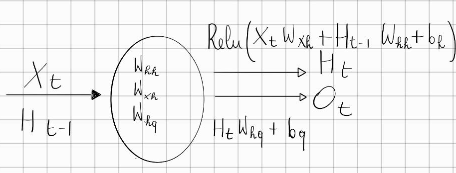
RNNs are neural networks with hidden states: the neural network takes as input both the current word x_n and the current hidden state z_{n'1} and produces an output word y_n as well as the next state z_n of the hidden variable. Specifically, the calculation of the hidden layer output of the current time step is determined by the input of the current time step together with the hidden layer output of the previous time step H_t = \phi(X_t W_{xh} + H_{t-1}W_{hh} + b_h) In particular, we are introducing a new weight parameter W_{hh} \in R^{h \times h} to describe how to use the hidden layer output of the previous time step in the current time step. H_{t-1} is the hidden layer output from the previous step.
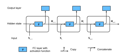
For time step t, the output of the output layer is similar to the computation in the MLP: O_t = H_t W_{hq} + b_q
16.2.1 Backpropagation through time
The error function consists of a sum over all output units of the error for each unit, in which each output unit has a softmax activation function along with an associated cross-entropy error function. During forward propagation, the activation values are propagated all the way from the first input in the sequence through to all the output nodes in the sequence, and error signals are then backpropagated along the same paths. This process is called backpropagation through time and in principle is straightforward. However, in practice, for very long sequences, training can be difficult due to the problems of vanishing gradients or exploding gradients: to see why this happens, let’s compute the derivative of the loss L with respect to the hidden-to-hidden weights W_{hh} \dfrac{\partial L}{\partial W_{hh}} = \dfrac{\partial}{\partial W_{hh}} \sum_{t=1}^T l(y_t, W_{hq} \cdot f(W_{hh} h_{t-1} + b_h) + b_q) \dfrac{\partial L_t}{\partial W_{hh}} = \sum_{k = 1}^t \dfrac{\partial L_t}{\partial h_t} \dfrac{\partial h_t}{\partial h_{k}} \dfrac{\partial h_{k}}{\partial W_{hh}} We notice that to compute the gradient at time step t we need to consider the influence of W_{hh} on every hidden state before h_t. This leads to \dfrac{\partial h_t}{\partial h_k} = \dfrac{\partial h_t}{\partial h_{t-1}} \dfrac{\partial h_{t-1}}{\partial h_{t-2}} \dots \dfrac{\partial h_{k+1}}{\partial h_k} = \prod_{i = k+1}^t \dfrac{\partial h_i}{\partial h_{i-1}} The single gradient \dfrac{\partial h_i}{\partial h_{i-1}} is computed by \mathbf{h}_i = f(\mathbf{h}_{i-1} \mathbf{W}_{hh} + \dots) \frac{\partial \mathbf{h}_i}{\partial \mathbf{h}_{i-1}} = \frac{\partial f(\mathbf{z}_i)}{\partial \mathbf{z}_i} \frac{\partial \mathbf{z}_i}{\partial \mathbf{h}_{i-1}} = \text{diag}(f'(\mathbf{z}_i)) \cdot \mathbf{W}_{hh}^T Given the previous product, we notice that we will multiply W_{hh} with itself t-k times, leading to very large powers of W_{hh}^T. In it, eigenvalues smaller than 1 vanish and eigenvalues larger than 1 diverge: A^2v = A(Av) = A(\lambda v) = \lambda(Av) = \lambda(\lambda v) = \lambda^2 v In general, A^n v = \lambda^n v. This is numerically unstable, which manifests itself in the form of vanishing and exploding gradients. One way to address this is to truncate the time steps at a computationally convenient size.
16.3 Long Short-Term Memory
The LSTM introduces an intermediate type of storage via the memory cell. Each memory cell is equipped with an internal state and a number of multiplicative gates that determine whether a given input should impact the internal state (input gate), whether the internal state should be flushed to 0 (forget gate), and whether the internal state of a given neuron should be allowed to impact the cell’s output (output gate). The key distinction between RNNs and LSTMs is that we have dedicated mechanisms for when a hidden state should be updated and also for when it should be reset.
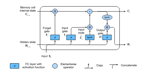
- Forget gate: F_t = \sigma(X_t W_{xf} + H_{t-1}W_{hf} + b_f)
- Input gate: I_t = \sigma(X_t W_{xi} + H_{t-1}W_{hi} + b_i)
- Output gate: O_t = \sigma(X_t W_{xo} + H_{t-1}W_{ho} + b_o)
- Input node: \hat{C_t} = \tanh(X_t W_{xc} + H_{t-1} W_{hc} + b_c)
So we need to find the weights:
- W_{xf} from input data to forget gate
- W_{xi} from input data to input gate
- W_{xo} from input data to output gate
- W_{xc} from input data to input node
- W_{hf} from hidden state to forget gate
- W_{hi} from hidden state to input gate
- W_{ho} from hidden state to output gate
- W_{hc} from hidden state to input node
To update the internal state we do
C_t = F_t \odot C_{t-1} + I_t \odot \hat{C_t}
In this way the input gates and the forget gates give the model the flexibility of being able to learn when to keep this value unchanged and when to perturb it in response to subsequent inputs.
To compute the output (=hidden state) we do H_{t} = O_t \odot \tanh(C_{t}) Whenever the output gate is close to 1, we allow the memory cell internal state to impact the subsequent layers uninhibited, whereas for output gate values close to 0, we prevent the current memory from impacting other layers of the network at the current time step.
16.4 Gated Recurrent Units (GRU)
GRUs are faster to compute than LSTMs. The LSTM’s three gates are replaced by the reset gate and the update gate. R_t = \sigma (X_t W_{xr} + H_{t-1}W_{hr} + b_r) Z_t = \sigma (X_t W_{xz} + H_{t-1}W_{hz} + b_z)
We integrate the reset gate with the hidden state at time step t - 1 computing a candidate hidden state (since we still need to incorporate the action of the update gate) \hat{H_t} = tanh(X_t W_{xh} + (R_t \odot H_{t-1}) W_{hh} + b_h)
Whenever R_t entries are close to 1, we recover a vanilla RNN, for all entries that are close to 0, the candidate hidden state is the result of a multi-layer perceptron: any pre-existing hidden state is reset to defaults.
The update gate can be used by taking the elementwise convex combinations of H_{t-1} and \hat{H_t}
H_t = Z_t \odot H_{t-1} + (1- Z_t) \odot \hat{H_t}
Whenever the update gate Z_t is close to 1, we simply retain the old state, skipping time step t.
Whenever Z_t is close to 0, the new latent state H_t approaches the candidate latent state \hat{H_t}.
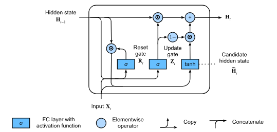
- Reset gates help capture short-term dependencies in sequences
- Update gates help capture long-term dependencies in sequences.
16.5 Deep Recurrent Neural Network
The way to create deep RNNs is simple: we stack the RNNs on top of each other. Given a sequence of length T, the first RNN produces a sequence of outputs, also of length T. These, in turn constitute the inputs to the next RNN layer. Any RNN cell at each time step depends on the same layer’s value at the previous time step and the previous layer’s value at the same time step.
Setting H_t^{(0)} = X_t, the hidden state of the l^{th} hidden layer that uses the activation function \phi_l is calculated as follows:
H_t ^{(l)} = \phi_l(H_t^{(l-1)} W_{xh}^{(l)} + H_{t- 1}^{(l)} W_{hh}^{(l)} + b_{h}^{(l)}) At the end, the output layer is based on the hidden state of the final L^{th} hidden layer: O_t = H_t^{(L)} W_{hq} + b_q
16.6 Bidirectional Recurrent Neural Networks
We simply implement two unidirectional RNN layers chained together in opposite directions and acting on the same input. For the first RNN layer, the first input is x_1 and the last input is x_T, but for the second RNN layer, the first input is x_T and the last input is x_1. To produce the output we simply concatenate together the corresponding outputs of the two underlying RNN layers, obtaining hidden states H_t \in R^{n \times 2h} instead of H_t \in R^{n\times h} as before.
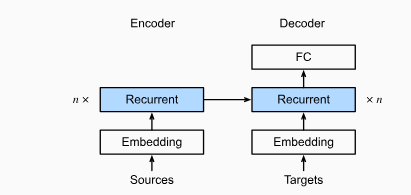
16.7 Sequence-to-Sequence models
In so-called sequence-to-sequence problems such as machine translation, where inputs and outputs each consist of variable-length unaligned sequences, we generally rely on encoder-decoder architectures. The encoder RNN will take a variable-length sequence as input and transform it into a fixed-shape hidden state. Then to generate the output sequence, one token at a time, the decoder model, consisting of a separate RNN, will predict each successive target token given both the input sequence and the preceding tokens in the output. During training, the decoder will typically be conditioned upon the preceding tokens in the official ‘ground truth’ label. However, at test time, we will want to condition each output of the decoder on the tokens already predicted.
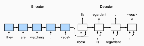
- Encoder: the input sequence is x_1, \ldots, x_T, such that x_t is the t^{th} token. At time step t, the RNN creates the current hidden state h_t based on x_t and h_{t-1}. The output of the encoder is a series of hidden states, that becomes a context vector passing through a function q:
c = q(h_1, \ldots, h_T)
- Decoder: given a target output sequence y_1, ..., y_T for each time step t, the decoder assigns a predicted probability to each possible token occurring at step y_{t+1} conditioned upon the previous tokens in the target and the context variable c
P(y_{t+1} | y_1, ... y_t, c)
To predict y_{t+1} the RNN decoder takes the previous step’s target token y_t, the hidden RNN state from the previous time step s_{t-1}, and the context variable c as input, and transforms them into the hidden state s_t at the current time step
s_t = g(y_{t-1}, c, s_{t-1})
After obtaining the hidden state of the decoder, we can use an output layer and the softmax operation to compute the predictive distribution p(y_{t+1} | y_1, ... y_t, c) over the subsequent output token t+1.
While running the encoder on the input sequence is relatively straightforward, handling the input and output of the decoder requires more care. The most common approach is called teacher forcing: we force the system to use the gold target token from training as the next input x_{t+1}, rather than allowing it to rely on the (possibly erroneous) decoder output y_t . This speeds up training.
16.7.1 Beam Search and Greedy Search
- Greedy Search: at any time step t, we simply select the token with the highest conditional probability
y_t = \argmax_{y \in \mathcal{Y}} P(y | y_1, ..., y_{t- 1}, c)
- Beam search: at time step 1, we select the k tokens with the highest predicted probabilities. Each of them will be the first token of k candidate output sequences, respectively. At each subsequent time step, based on the k candidate output sequences at the previous time step, we continue to select k candidate output sequences with the highest predicted probabilities.
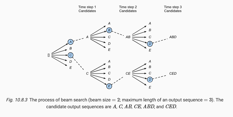
In the end, we choose the output sequence which maximizes the following score
\dfrac{1}{L^{\alpha}} \log P(y_1, ..., y_L | c) = \dfrac{1}{L^{\alpha}} \sum_{t = 1}^L \log P(y_t | y_1, ... y_{t-1}, c)
L is the length of the final candidate sequence and \alpha is usually set to 0.75. Since a longer sequence has more logarithmic terms in the summation, the term L^{\alpha} in the denominator penalizes long sequences. Greedy search can be treated as a special case of beam search where k = 1.